What Is A Low Pass Filter Currnet

Blazon of signal filter

A low-pass filter is a filter that passes signals with a frequency lower than a selected cutoff frequency and attenuates signals with frequencies higher than the cutoff frequency. The exact frequency response of the filter depends on the filter pattern. The filter is sometimes called a high-cut filter, or treble-cut filter in sound applications. A low-pass filter is the complement of a loftier-pass filter.

In optics, loftier-laissez passer and low-pass may have unlike meanings, depending on whether referring to frequency or wavelength of low-cal, since these variables are inversely related. High-pass frequency filters would act as low-laissez passer wavelength filters, and vice versa. For this reason it is a adept practise to refer to wavelength filters as brusk-laissez passer and long-laissez passer to avoid defoliation, which would correspond to high-laissez passer and depression-pass frequencies.^[1]

Depression-laissez passer filters be in many different forms, including electronic circuits such as a hiss filter used in audio, anti-aliasing filters for conditioning signals prior to analog-to-digital conversion, digital filters for smoothing sets of data, acoustic barriers, blurring of images, and then on. The moving average operation used in fields such every bit finance is a particular kind of low-pass filter, and tin can be analyzed with the same point processing techniques as are used for other low-pass filters. Depression-pass filters provide a smoother form of a signal, removing the short-term fluctuations and leaving the longer-term trend.

Filter designers will often use the low-laissez passer form as a prototype filter. That is, a filter with unity bandwidth and impedance. The desired filter is obtained from the prototype by scaling for the desired bandwidth and impedance and transforming into the desired bandform (that is depression-pass, high-pass, band-laissez passer or band-stop).

Examples [edit]

Examples of depression-laissez passer filters occur in acoustics, optics and electronics.

A stiff concrete barrier tends to reverberate college sound frequencies, and and then acts as an acoustic low-pass filter for transmitting audio. When music is playing in another room, the depression notes are easily heard, while the high notes are attenuated.

An optical filter with the aforementioned function can correctly be chosen a depression-pass filter, but conventionally is called a longpass filter (low frequency is long wavelength), to avoid defoliation.^[two]

In an electronic low-pass RC filter for voltage signals, high frequencies in the input signal are attenuated, just the filter has little attenuation below the cutoff frequency adamant by its RC fourth dimension abiding. For current signals, a like excursion, using a resistor and capacitor in parallel, works in a similar manner. (Come across current divider discussed in more item below.)

Electronic low-pass filters are used on inputs to subwoofers and other types of loudspeakers, to block high pitches that they cannot efficiently reproduce. Radio transmitters utilise low-pass filters to block harmonic emissions that might interfere with other communications. The tone knob on many electric guitars is a depression-pass filter used to reduce the amount of treble in the sound. An integrator is another time abiding low-laissez passer filter.^[3]

Telephone lines fitted with DSL splitters use low-pass and loftier-pass filters to separate DSL and POTS signals sharing the same pair of wires.^{[4] [5]}

Low-laissez passer filters besides play a significant office in the sculpting of sound created by analogue and virtual analogue synthesisers. See subtractive synthesis.

A low-pass filter is used as an anti-aliasing filter prior to sampling and for reconstruction in digital-to-analog conversion.

Ideal and real filters [edit]

The gain-magnitude frequency response of a first-gild (1-pole) low-pass filter. Ability gain is shown in decibels (i.e., a 3 dB decline reflects an boosted one-half-power attenuation). Angular frequency is shown on a logarithmic scale in units of radians per second.

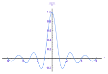
An ideal low-pass filter completely eliminates all frequencies above the cutoff frequency while passing those below unchanged; its frequency response is a rectangular office and is a brick-wall filter. The transition region present in practical filters does not exist in an ideal filter. An platonic low-pass filter can be realized mathematically (theoretically) by multiplying a point by the rectangular function in the frequency domain or, equivalently, convolution with its impulse response, a sinc function, in the time domain.

Nevertheless, the platonic filter is impossible to realize without likewise having signals of infinite extent in time, and so more often than not needs to be approximated for real ongoing signals, considering the sinc function's support region extends to all by and time to come times. The filter would therefore demand to have space delay, or noesis of the infinite future and by, in lodge to perform the convolution. It is effectively realizable for pre-recorded digital signals by bold extensions of zero into the by and time to come, or more typically past making the betoken repetitive and using Fourier analysis.

Existent filters for real-time applications approximate the ideal filter by truncating and windowing the infinite impulse response to make a finite impulse response; applying that filter requires delaying the betoken for a moderate catamenia of fourth dimension, allowing the computation to "see" a little scrap into the futurity. This delay is manifested as phase shift. Greater accurateness in approximation requires a longer filibuster.

An ideal low-pass filter results in ringing artifacts via the Gibbs miracle. These can be reduced or worsened past choice of windowing office, and the blueprint and choice of real filters involves understanding and minimizing these artifacts. For instance, "simple truncation [of sinc] causes severe ringing artifacts," in signal reconstruction, and to reduce these artifacts one uses window functions "which drib off more smoothly at the edges."^[half-dozen]

The Whittaker–Shannon interpolation formula describes how to use a perfect depression-pass filter to reconstruct a continuous signal from a sampled digital signal. Real digital-to-analog converters use existent filter approximations.

Time response [edit]

The fourth dimension response of a low-pass filter is found by solving the response to the simple low-laissez passer RC filter.

Using Kirchhoff'due south Laws we make it at the differential equation^[7]

${\displaystyle v_{\text{out}}(t)=v_{\text{in}}(t)-RC{\frac {\operatorname {d} v_{\text{out}}}{\operatorname {d} t}}}$

Step input response example [edit]

If nosotros let ${\displaystyle v_{\text{in}}(t)}$ exist a footstep function of magnitude ${\displaystyle V_{i}}$ then the differential equation has the solution^[viii]

${\displaystyle v_{\text{out}}(t)=V_{i}(ane-east^{-\omega _{0}t}),}$

where ${\displaystyle \omega _{0}={ane \over RC}}$ is the cutoff frequency of the filter.

Frequency response [edit]

The almost mutual style to characterize the frequency response of a circuit is to find its Laplace transform^[7] transfer function, ${\displaystyle H(due south)={V_{\rm {out}}(southward) \over V_{\rm {in}}(s)}}$ . Taking the Laplace transform of our differential equation and solving for ${\displaystyle H(s)}$ we become

${\displaystyle H(s)={V_{\rm {out}}(s) \over V_{\rm {in}}(s)}={\omega _{0} \over (southward+\omega _{0})}}$

Difference equation through discrete time sampling [edit]

A discrete difference equation is easily obtained by sampling the step input response higher up at regular intervals of ${\displaystyle nT}$ where ${\displaystyle n=0,ane,...}$ and ${\displaystyle T}$ is the time between samples. Taking the divergence between two consecutive samples we accept

${\displaystyle v_{\rm {out}}(nT)-v_{\rm {out}}((n-1)T)=V_{i}(one-due east^{-\omega _{0}nT})-V_{i}(1-e^{-\omega _{0}((due north-one)T)})}$

Solving for ${\displaystyle v_{\rm {out}}(nT)}$ nosotros get

${\displaystyle v_{\rm {out}}(nT)=\beta v_{\rm {out}}((northward-1)T)+(1-\beta )V_{i}}$

Where ${\displaystyle \beta =e^{-\omega _{0}T}}$

Using the annotation ${\displaystyle V_{n}=v_{\rm {out}}(nT)}$ and ${\displaystyle v_{n}=v_{\rm {in}}(nT)}$ , and substituting our sampled value, ${\displaystyle v_{n}=V_{i}}$ , we get the difference equation

${\displaystyle V_{north}=\beta V_{n-1}+(1-\beta )v_{northward}}$

Error analysis [edit]

Comparing the reconstructed output betoken from the divergence equation, ${\displaystyle V_{n}=\beta V_{n-1}+(1-\beta )v_{n}}$ , to the step input response, ${\displaystyle v_{\text{out}}(t)=V_{i}(1-east^{-\omega _{0}t})}$ , we find that there is an verbal reconstruction (0% mistake). This is the reconstructed output for a time invariant input. Nonetheless, if the input is time variant, such as ${\displaystyle v_{\text{in}}(t)=V_{i}\sin(\omega t)}$ , this model approximates the input bespeak every bit a series of pace functions with duration ${\displaystyle T}$ producing an error in the reconstructed output signal. The error produced from time variant inputs is difficult to quantify^{[ citation needed ]} but decreases as ${\displaystyle T\rightarrow 0}$ .

Detached-time realization [edit]

For another method of conversion from continuous- to discrete-time, come across Bilinear transform.

Many digital filters are designed to requite low-pass characteristics. Both infinite impulse response and finite impulse response depression pass filters besides every bit filters using Fourier transforms are widely used.

Simple space impulse response filter [edit]

The consequence of an infinite impulse response depression-pass filter can be simulated on a computer by analyzing an RC filter'southward behavior in the fourth dimension domain, and so discretizing the model.

From the excursion diagram to the right, co-ordinate to Kirchhoff'south Laws and the definition of capacitance:

${\displaystyle v_{\text{in}}(t)-v_{\text{out}}(t)=R\;i(t)}$

(V)

${\displaystyle Q_{c}(t)=C\,v_{\text{out}}(t)}$

(Q)

${\displaystyle i(t)={\frac {\operatorname {d} Q_{c}}{\operatorname {d} t}}}$

(I)

where ${\displaystyle Q_{c}(t)}$ is the charge stored in the capacitor at time t. Substituting equation Q into equation I gives ${\displaystyle i(t)\;=\;C{\frac {\operatorname {d} v_{\text{out}}}{\operatorname {d} t}}}$ , which can be substituted into equation Five so that

${\displaystyle v_{\text{in}}(t)-v_{\text{out}}(t)=RC{\frac {\operatorname {d} v_{\text{out}}}{\operatorname {d} t}}.}$

This equation can exist discretized. For simplicity, assume that samples of the input and output are taken at evenly spaced points in time separated by ${\displaystyle \Delta _{T}}$ time. Let the samples of ${\displaystyle v_{\text{in}}}$ exist represented by the sequence ${\displaystyle (x_{ane},\,x_{2},\,\ldots ,\,x_{n})}$ , and let ${\displaystyle v_{\text{out}}}$ be represented by the sequence ${\displaystyle (y_{one},\,y_{two},\,\ldots ,\,y_{due north})}$ , which correspond to the same points in fourth dimension. Making these substitutions,

${\displaystyle x_{i}-y_{i}=RC\,{\frac {y_{i}-y_{i-i}}{\Delta _{T}}}.}$

Rearranging terms gives the recurrence relation

${\displaystyle y_{i}=\overbrace {x_{i}\left({\frac {\Delta _{T}}{RC+\Delta _{T}}}\right)} ^{\text{Input contribution}}+\overbrace {y_{i-1}\left({\frac {RC}{RC+\Delta _{T}}}\right)} ^{\text{Inertia from previous output}}.}$

That is, this discrete-time implementation of a simple RC low-pass filter is the exponentially weighted moving average

${\displaystyle y_{i}=\alpha x_{i}+(1-\alpha )y_{i-1}\qquad {\text{where}}\qquad \blastoff :={\frac {\Delta _{T}}{RC+\Delta _{T}}}.}$

By definition, the smoothing cistron ${\displaystyle 0\;\leq \;\alpha \;\leq \;1}$ . The expression for α yields the equivalent time abiding RC in terms of the sampling period ${\displaystyle \Delta _{T}}$ and smoothing gene α,

${\displaystyle RC=\Delta _{T}\left({\frac {1-\alpha }{\alpha }}\right).}$

Recalling that

${\displaystyle f_{c}={\frac {1}{2\pi RC}}}$ so ${\displaystyle RC={\frac {ane}{ii\pi f_{c}}},}$

note α and ${\displaystyle f_{c}}$ are related by,

${\displaystyle \alpha ={\frac {two\pi \Delta _{T}f_{c}}{2\pi \Delta _{T}f_{c}+i}}}$

and

${\displaystyle f_{c}={\frac {\alpha }{(1-\alpha )2\pi \Delta _{T}}}.}$

If α=0.5, so the RC time abiding is equal to the sampling menses. If ${\displaystyle \alpha \;\ll \;0.five}$ , and then RC is significantly larger than the sampling interval, and ${\displaystyle \Delta _{T}\;\approx \;\alpha RC}$ .

The filter recurrence relation provides a mode to determine the output samples in terms of the input samples and the preceding output. The following pseudocode algorithm simulates the issue of a low-pass filter on a series of digital samples:

// Render RC low-pass filter output samples, given input samples, // time interval          dt, and fourth dimension constant          RC          office          lowpass(real[0..n]          x,          existent          dt,          real          RC)          var          real[0..northward]          y          var          existent          α := dt / (RC + dt)     y[0] := α * ten[0]          for          i          from          ane          to          north         y[i] := α * x[i] + (ane-α) * y[i-one]          return          y        

The loop that calculates each of the n outputs can be refactored into the equivalent:

          for          i          from          i          to          n         y[i] := y[i-one] + α * (x[i] - y[i-1])        

That is, the change from one filter output to the next is proportional to the difference between the previous output and the side by side input. This exponential smoothing property matches the exponential decay seen in the continuous-fourth dimension system. As expected, every bit the fourth dimension constant RC increases, the discrete-time smoothing parameter ${\displaystyle \alpha }$ decreases, and the output samples ${\displaystyle (y_{1},\,y_{2},\,\ldots ,\,y_{north})}$ respond more slowly to a change in the input samples ${\displaystyle (x_{ane},\,x_{2},\,\ldots ,\,x_{n})}$ ; the system has more inertia. This filter is an infinite-impulse-response (IIR) single-pole depression-pass filter.

Finite impulse response [edit]

Finite-impulse-response filters can exist congenital that approximate to the sinc function time-domain response of an platonic sharp-cutoff depression-pass filter. For minimum distortion the finite impulse response filter has an unbounded number of coefficients operating on an unbounded signal. In practice, the time-domain response must be fourth dimension truncated and is ofttimes of a simplified shape; in the simplest case, a running average can be used, giving a square fourth dimension response.^[9]

Fourier transform [edit]

For non-realtime filtering, to achieve a low pass filter, the entire point is usually taken as a looped signal, the Fourier transform is taken, filtered in the frequency domain, followed by an inverse Fourier transform. Merely O(n log(north)) operations are required compared to O(n²) for the fourth dimension domain filtering algorithm.

This tin can as well sometimes be washed in real-fourth dimension, where the signal is delayed long enough to perform the Fourier transformation on shorter, overlapping blocks.

Continuous-fourth dimension realization [edit]

Plot of the gain of Butterworth depression-pass filters of orders 1 through 5, with cutoff frequency ${\displaystyle \omega _{0}=i}$ . Note that the slope is 20n dB/decade where n is the filter order.

At that place are many unlike types of filter circuits, with different responses to changing frequency. The frequency response of a filter is generally represented using a Bode plot, and the filter is characterized by its cutoff frequency and rate of frequency rolloff. In all cases, at the cutoff frequency, the filter attenuates the input power by half or 3 dB. So the guild of the filter determines the amount of additional attenuation for frequencies higher than the cutoff frequency.

• A get-go-club filter, for example, reduces the signal amplitude by half (so ability reduces by a gene of 4, or six dB), every time the frequency doubles (goes up one octave); more than precisely, the power rolloff approaches 20 dB per decade in the limit of loftier frequency. The magnitude Bode plot for a offset-order filter looks like a horizontal line beneath the cutoff frequency, and a diagonal line to a higher place the cutoff frequency. There is also a "knee joint curve" at the boundary between the two, which smoothly transitions betwixt the two direct line regions. If the transfer office of a first-social club low-laissez passer filter has a zero also equally a pole, the Bode plot flattens out again, at some maximum attenuation of high frequencies; such an result is caused for case by a lilliputian bit of the input leaking effectually the one-pole filter; this i-pole–one-nil filter is still a kickoff-social club depression-pass. See Pole–cypher plot and RC circuit.
• A 2nd-order filter attenuates high frequencies more than steeply. The Bode plot for this type of filter resembles that of a offset-order filter, except that it falls off more quickly. For instance, a 2nd-order Butterworth filter reduces the signal aamplitude to one fourth its original level every fourth dimension the frequency doubles (so power decreases by 12 dB per octave, or 40 dB per decade). Other all-pole second-order filters may roll off at different rates initially depending on their Q factor, merely approach the same final rate of 12 dB per octave; as with the first-order filters, zeroes in the transfer function tin can change the high-frequency asymptote. See RLC circuit.
• Third- and college-order filters are defined similarly. In general, the final rate of power rolloff for an order- northward all-pole filter is vin dB per octave (20due north dB per decade).

On whatever Butterworth filter, if ane extends the horizontal line to the right and the diagonal line to the upper-left (the asymptotes of the role), they intersect at exactly the cutoff frequency. The frequency response at the cutoff frequency in a first-order filter is 3 dB below the horizontal line. The various types of filters (Butterworth filter, Chebyshev filter, Bessel filter, etc.) all have dissimilar-looking knee joint curves. Many 2nd-order filters have "peaking" or resonance that puts their frequency response at the cutoff frequency above the horizontal line. Furthermore, the actual frequency where this peaking occurs can be predicted without calculus, equally shown by Cartwright^[10] et al. For third-order filters, the peaking and its frequency of occurrence can also exist predicted without calculus as shown past Cartwright^[11] et al. Run into electronic filter for other types.

The meanings of 'low' and 'high'—that is, the cutoff frequency—depend on the characteristics of the filter. The term "low-pass filter" just refers to the shape of the filter'south response; a high-laissez passer filter could be built that cuts off at a lower frequency than any low-pass filter—information technology is their responses that prepare them apart. Electronic circuits can be devised for whatever desired frequency range, right upward through microwave frequencies (above i GHz) and college.

Laplace annotation [edit]

Continuous-time filters can too exist described in terms of the Laplace transform of their impulse response, in a way that lets all characteristics of the filter be easily analyzed by considering the pattern of poles and zeros of the Laplace transform in the circuitous airplane. (In discrete time, one tin similarly consider the Z-transform of the impulse response.)

For case, a start-society depression-laissez passer filter can be described in Laplace notation equally:

${\displaystyle {\frac {\text{Output}}{\text{Input}}}=Chiliad{\frac {1}{\tau due south+ane}}}$

where south is the Laplace transform variable, τ is the filter time constant, and K is the proceeds of the filter in the passband.

Electronic low-pass filters [edit]

Commencement order [edit]

RC filter [edit]

Passive, first social club low-laissez passer RC filter

One simple low-laissez passer filter circuit consists of a resistor in series with a load, and a capacitor in parallel with the load. The capacitor exhibits reactance, and blocks low-frequency signals, forcing them through the load instead. At higher frequencies the reactance drops, and the capacitor effectively functions every bit a short circuit. The combination of resistance and capacitance gives the time constant of the filter ${\displaystyle \tau \;=\;RC}$ (represented by the Greek alphabetic character tau). The pause frequency, besides called the turnover frequency, corner frequency, or cutoff frequency (in hertz), is adamant past the time constant:

${\displaystyle f_{\mathrm {c} }={ane \over ii\pi \tau }={1 \over two\pi RC}}$

or equivalently (in radians per second):

${\displaystyle \omega _{\mathrm {c} }={1 \over \tau }={1 \over RC}}$

This circuit may be understood by considering the time the capacitor needs to charge or discharge through the resistor:

• At low frequencies, at that place is plenty of time for the capacitor to accuse upwardly to practically the same voltage equally the input voltage.
• At high frequencies, the capacitor merely has time to charge upwards a small amount earlier the input switches direction. The output goes upward and down only a minor fraction of the amount the input goes upwardly and down. At double the frequency, there's simply time for it to charge up half the amount.

Some other fashion to understand this excursion is through the concept of reactance at a detail frequency:

• Since direct electric current (DC) cannot flow through the capacitor, DC input must flow out the path marked ${\displaystyle V_{\mathrm {out} }}$ (analogous to removing the capacitor).
• Since alternating current (AC) flows very well through the capacitor, virtually besides as it flows through solid wire, AC input flows out through the capacitor, effectively short circuiting to ground (coordinating to replacing the capacitor with just a wire).

The capacitor is not an "on/off" object (like the block or laissez passer fluidic explanation above). The capacitor variably acts betwixt these two extremes. It is the Bode plot and frequency response that prove this variability.

RL filter [edit]

A resistor–inductor circuit or RL filter is an electrical circuit composed of resistors and inductors driven past a voltage or electric current source. A beginning order RL circuit is composed of 1 resistor and 1 inductor and is the simplest type of RL circuit.

A kickoff society RL circuit is 1 of the simplest analogue infinite impulse response electronic filters. Information technology consists of a resistor and an inductor, either in series driven past a voltage source or in parallel driven by a current source.

Second gild [edit]

RLC filter [edit]

RLC excursion as a depression-pass filter

An RLC circuit (the letters R, L and C can exist in a dissimilar sequence) is an electric excursion consisting of a resistor, an inductor, and a capacitor, continued in series or in parallel. The RLC part of the name is due to those letters being the usual electrical symbols for resistance, inductance and capacitance respectively. The circuit forms a harmonic oscillator for current and volition resonate in a similar way as an LC circuit will. The master divergence that the presence of the resistor makes is that whatsoever oscillation induced in the circuit will die abroad over time if it is not kept going by a source. This upshot of the resistor is called damping. The presence of the resistance also reduces the pinnacle resonant frequency somewhat. Some resistance is unavoidable in real circuits, even if a resistor is non specifically included as a component. An ideal, pure LC circuit is an abstraction for the purpose of theory.

At that place are many applications for this circuit. They are used in many different types of oscillator circuits. Another important awarding is for tuning, such as in radio receivers or boob tube sets, where they are used to select a narrow range of frequencies from the ambient radio waves. In this role the circuit is often referred to as a tuned circuit. An RLC circuit can be used equally a band-pass filter, band-cease filter, low-pass filter or high-laissez passer filter. The RLC filter is described as a second-order circuit, meaning that any voltage or current in the circuit tin be described by a second-society differential equation in circuit analysis.

Higher order passive filters [edit]

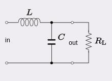
College order passive filters can also be constructed (see diagram for a third order example).

A tertiary-lodge low-laissez passer filter (Cauer topology). The filter becomes a Butterworth filter with cutoff frequency ω_c=1 when (for example) C_ii=4/three farad, R₄=1 ohm, 50₁=3/2 henry and L₃=1/2 henry.

Active electronic realization [edit]

An agile low-pass filter

Another type of electric excursion is an agile low-pass filter.

In the operational amplifier circuit shown in the figure, the cutoff frequency (in hertz) is defined as:

${\displaystyle f_{\text{c}}={\frac {1}{2\pi R_{2}C}}}$

or equivalently (in radians per 2d):

${\displaystyle \omega _{\text{c}}={\frac {1}{R_{2}C}}}$

The proceeds in the passband is −R _two/R ₁, and the stopband drops off at −6 dB per octave (that is −xx dB per decade) as information technology is a first-order filter.

Run into also [edit]

• Baseband

References [edit]

1. ^ Long Laissez passer Filters and Short Pass Filters Information , retrieved 2017-10-04
2. ^ Long Pass Filters and Brusk Pass Filters Information , retrieved 2017-x-04
3. ^ Sedra, Adel; Smith, Kenneth C. (1991). Microelectronic Circuits, 3 ed . Saunders College Publishing. p. threescore. ISBN0-03-051648-X.
4. ^ "ADSL filters explained". Epanorama.cyberspace. Retrieved 2013-09-24 .
5. ^ "Domicile Networking – Local Area Network". Pcweenie.com. 2009-04-12. Archived from the original on 2013-09-27. Retrieved 2013-09-24 .
6. ^ Mastering Windows: Improving Reconstruction
7. ^ ^{a b} Hayt, William H., Jr. and Kemmerly, Jack E. (1978). Engineering Circuit Assay. New York: McGRAW-Hill Volume COMPANY. pp. 211–224, 684–729. {{cite volume}}: CS1 maint: multiple names: authors list (link)
8. ^ Boyce, William and DiPrima, Richard (1965). Elementary Differential Equations and Boundary Value Problems. New York: JOHN WILEY & SONS. pp. 11–24. {{cite book}}: CS1 maint: multiple names: authors listing (link)
9. ^ Whilmshurst, T H (1990) Indicate recovery from noise in electronic instrumentation. ISBN 9780750300582
10. ^ K. V. Cartwright, P. Russell and Eastward. J. Kaminsky,"Finding the maximum magnitude response (gain) of 2nd-gild filters without calculus," Lat. Am. J. Phys. Educ. Vol. half-dozen, No. iv, pp. 559–565, 2012.
11. ^ Cartwright, Grand. 5.; P. Russell; E. J. Kaminsky (2013). "Finding the maximum and minimum magnitude responses (gains) of third-order filters without calculus" (PDF). Lat. Am. J. Phys. Educ. vii (four): 582–587.

External links [edit]

• Depression Laissez passer Filter java simulator
• ECE 209: Review of Circuits as LTI Systems, a short primer on the mathematical assay of (electric) LTI systems.
• ECE 209: Sources of Phase Shift, an intuitive explanation of the source of phase shift in a depression-pass filter. Likewise verifies simple passive LPF transfer function by means of trigonometric identity.

What Is A Low Pass Filter Currnet,

Source: https://en.wikipedia.org/wiki/Low-pass_filter

Posted by: arneybadeltudy.blogspot.com

Share this post